Tölvera v0.1.0 API Guide
This guide provides an overview of the Tölvera v0.1.0 API:
The v0.2.0 API will be different, so everything here is subject to change.
Please share your feedback on our Discord.
Overview of Features
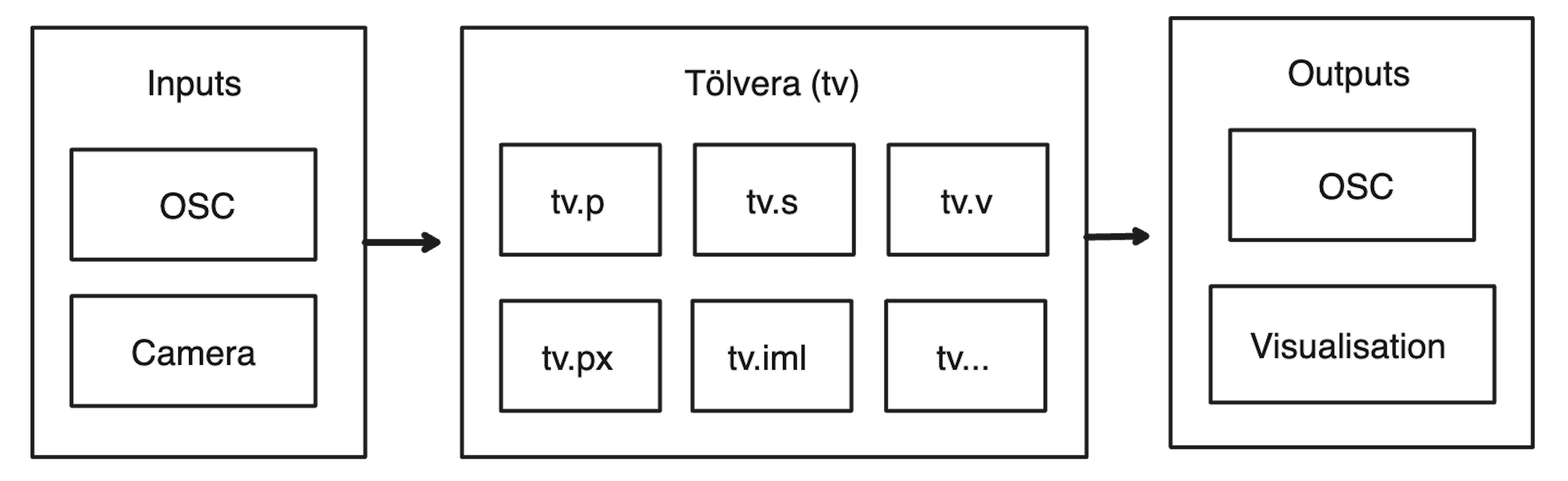
tv.v: a collection of "vera" (beings) including Move, Flock, Slime and Swarm, with more being continuously added. Vera can be combined and composed in various ways.tv.p: extensible particle system. Particles are divided into multiple species, where each species has a unique relationship with every other species, including itselftv.s: n-dimensional state structures that can be used by "vera", including built-in OSC and IML creation (see below).tv.px: drawing library including various shapes and blend modes, styled similarly to p5.js etc.tv.osc: Open Sound Control (OSC) via iipyper, including automated export of OSC schemas to JSON, XML, Pure Data (Pd), Max/MSP (SuperCollider TBC).tv.iml: Interactive Machine Learning via anguilla.tv.ti: Taichi-based simulation and rendering engine. Can be run "headless" (without graphics).tv.cv: computer vision integration based on OpenCV and Mediapipe.
Program Structure
This example demonstrates the basic usage of Tölvera when used as a standalone Python script. It will display a window with a black background:
from tolvera import Tolvera, run

def main(**kwargs):
  tv = Tolvera(**kwargs)

  @tv.render
  def _():
      return tv.px

if __name__ == '__main__':
  run(main)
- First, we import the
Tolveraclass andrun()function from thetolveraPython package. - Then, a
def main()function takes in keyword arguments (**kwargs) from the command line. - Inside
def main(), we initialise aTolverainstance with the given**kwargs. - We use the
@tv.render()decorator to create the scene and render the pixels. - This function can be named anything (
def _()in the example), and is analagous toloop()in Arduino/Processing/p5.js andrender()in Bela, in that it will run in a loop until the user exits the program. - However,
def _()must return an instance ofPixels. - Often, these pixels will be the
Pixelsinstance belonging to theTolverainstance, accessed withtv.px. - Finally, we call
run()withdef main()as the argument.
Particles (tv.p) & Species (tv.s.species)
A central idea of Tölvera is the particle as a base unit of activity.
The particle system is a field of type Particle with these properties:
@ti.dataclass
class Particle:
  species: ti.i32
  active: ti.f32
  pos: ti.math.vec2
  vel: ti.math.vec2
  mass: ti.f32
  size: ti.f32
  speed: ti.f32
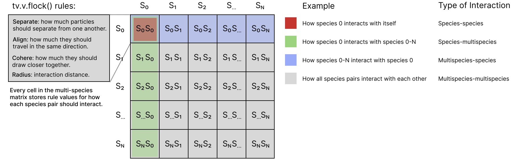
Particles are divided into species (represented as an integer), and species can have different relationships with each other, creating a matrix of species-species interactions.
This idea was inspired by Particle Life, and provides a simple means to mimic ecological complexity, even when using a single behaviour or model.
Species are implemented as multi-dimensional state (see below), which means all tv.v behaviour models can make use of the multispecies matrix.
State (tv.s)
To enable composition of behaviours, Tölvera features a global state dictionary.
State is n-dimensional and can be manipulated in parallel on the GPU.
Typical state shapes might be: (species, species) for multispecies rules, (particles) for individual particle states, and \pyi(particles, particles) for pairwise comparison of particles.
Assigning a dictionary to a variable after tv.s causes a new state to be instanced.
Here are two examples of state from tv.v.flock, showing the syntax of "name": (type, min, max) for each attribute, and some of the additional options which includes built-in randomisation:
tv.s.flock_s = { "state":
  {
    "separate": (ti.f32, 0.01, 1.0),
    "align": (ti.f32, 0.01, 1.0),
    "cohere": (ti.f32, 0.01, 1.0),
    "radius": (ti.f32, 0.01, 1.0),
  },
  "shape": (species, species),
  "osc": ("set"),
  "randomise": True
}

tv.s.flock_dist = {
  "state": {"dist": (ti.f32, 0.0, tv.x*2)},
  "shape": (particles, particles),
  "randomise": False
}
State is useful and interesting to visualise, for example drawing the particle distances that flock uses reveals hidden structure.
State can also be reused and combined with state from other models, to compose even more complex behaviour.
Vera (tv.v)
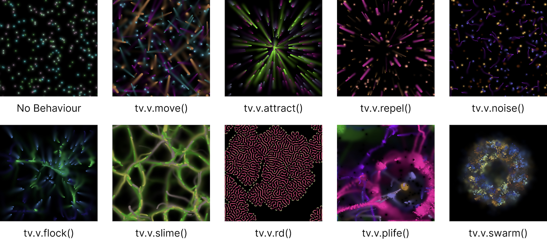
The image below shows some of the available behaviours and models in Tölvera. Some of these are inspired directly from open source code posted by the Taichi community - thank you!
Models can be used by calling them and passing particles to them, for example:
@tv.render
def _():
  tv.px.clear()
  tv.v.flock(tv.p)
  tv.v.plife(tv.p)
  tv.px.particles(tv.p, tv.s.species())
  return tv.px
In this case, the flock and plife (particle life) models are composed together to create a compound behaviour.
Models are also designed to be simple and concise internally to encourage users to understand them and make their own.
Simple behaviours like move can be stateless and implemented as single GPU kernels.
@ti.kernel
def move(p: ti.template()):
  for i in range(p.field.shape[0]):
    p1 = p.field[i]
    if p1.field[i].active == 0: continue
    p.field[i].pos += p1.vel * p1.speed
Models that use state are implemented as classes, that at minimum provide a step() method, where particles can be compared and states updated:
@ti.data_oriented
class MyVera:
  def __init__(self, tolvera, **kwargs):
    self.tv, self.kwargs = tolvera, kwargs
    self.C = CONSTS({...})
    self.tv.s.vera_s = {...} # state

  @ti.kernel
  def step(self, p):
    for i in range(p.shape[0]):
      for j in range(p.shape[1]):
        # compare p[i] & p[j]
        # update state, etc.
      p[i].pos += ... # update p[i]

  def __call__(self, p):
    self.step(p)
Step function inside tv.v:
@ti.kernel
def step(self, p: ti.template(), W: ti.f32):
  for i in range(p.shape[0]):
    p1 = p[i]
    if p1[i].active == 0: continue
    for j in range(p.shape[0]):
      p2 = p[j]
      if i == j & p2[j].active == 0: continue
      s = self.tv.s.vera_s[p1.species, p2.species]
      d = p1.pos - p2.pos
      if d < s.radius:
        # p1 & p2 are neighbours
    p[i].vel += W * ...
    p[i].pos += W * ...
Pixels (tv.px)
Tölvera has a drawing module that is similar in design to p5.js. This example draws a rectangle in the middle of the window:
import taichi as ti
from tolvera import Tolvera, run

def main(**kwargs):
    tv = Tolvera(**kwargs)

    @ti.kernel
    def draw():
        w = 100
        tv.px.rect(tv.x/2-w/2, tv.y/2-w/2, w, w, ti.Vector([1., 0., 0., 1.]))

    @tv.render
    def _():
        draw()
        return tv.px

if __name__ == '__main__':
    run(main)
It mainly features shape primitives and blend modes.
Pixels can also be thought of as fields and used as part of a vera, as tv.v.slime does to deposit particles onto a pheromone trail.
Due to this flexibility, drawing and visualisation can impact behaviour and create more mappings and feedback loops between model states.
GPU Programming (tv.ti)
Tölvera does most of its work on the GPU thanks to Taichi (tv.ti).
Taichi is a domain-specific language (DSL) embedded in Python that supports multiple backends (CUDA, OpenGL, Vulkan, Metal).
Taichi programs are distinguished by three levels of scope: regular Python scope, kernel scope (@ti.kernel) and function scope (@ti.func).
Python scope can call kernels, and kernels and functions can call functions.
In Taichi scope, top-level for loops are automatically parallelised.
It can also run headless (without a window), and provides a C runtime and ahead-of-time (AOT) compilation for deployment in non-Python programs.
It also interoperates with NumPy and PyTorch for ML integrations.
Open Sound Control (tv.osc)
OSC in Tölvera is handled by iipyper, a package specifically designed for working with artificial intelligence.
When creating state, OSC endpoints can be automatically added via the "osc" option.
For custom OSC endpoints, the tv.osc.map decorators can be used to add senders and receivers of different varieties.
Here are two examples, one of receiving two arguments x and y, and another of receiving a vector of length ten:
@tv.osc.map.receive_args(x=(0.,0.,1.), y=(0.,0.,1.), count=5)
def my_args(x: float, y: float):
  print(f"Receiving args: {x} {y}")

@tv.osc.map.receive_list(vector=(0.,0.,1.), length=10, count=5)
def my_list(vector: list[float]):
  print(f"Received list: {vector}")
The count decorator argument can be used to rate limit how often an endpoint's Python function runs, relative to the number of frames elapsing.
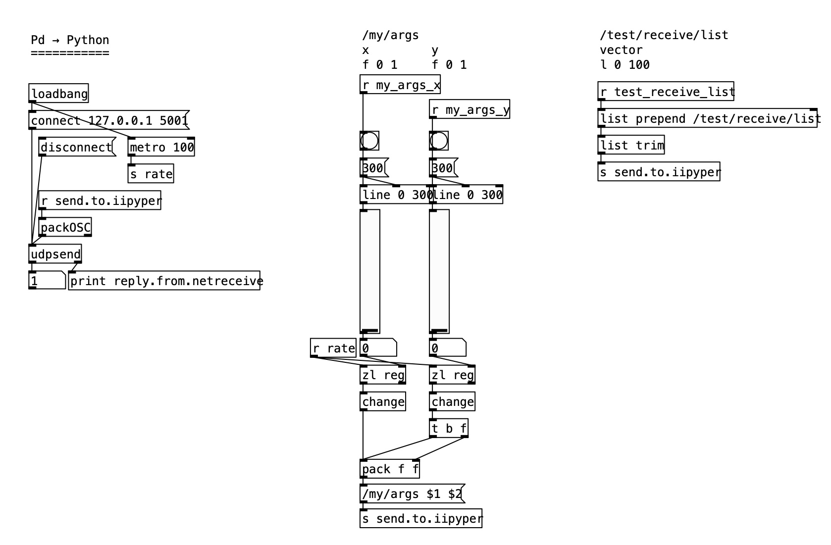
Tölvera OSC mappings can be exported to JSON and XML, and they can also generate patches for Max/MSP and Pure Data, enabling rapid integration with other software.
Interactive Machine Learning (tv.iml)
Interactive machine learning is achieved via the anguilla Python package.
Tölvera features a global dictionary of IML instances at tv.iml, similarly to state (tv.s).
IML can be used for a wide range of purposes in Tölvera, including creating internal feedback loops, for example between tv.v.flock's position and species rules states:
tv.iml.flock_p2flock_s = {
  'type': 'fun2fun',
  'size': (tv.s.flock_p.size, tv.s.flock_s.size),
  'io': (tv.s.flock_p.to_vec, tv.s.flock_s.from_vec)
}
The above example uses fun2fun, meaning the input and output methods specified in the io option will be run in the background by Tölvera.
These are to_vec and from_vec, built-in methods that serialise and deserialise state to/from 1D arrays making them suitable for use as IML input/output vectors.
To facilitate automatic routing of IML inputs and outputs, there are nine types in which the input and output can be either a vector, function or OSC endpoint:
vec2vec,
vec2fun,
vec2osc,
fun2vec,
fun2fun,
fun2osc,
osc2vec,
osc2fun,
and osc2osc.
Notably, these IML maps can be trained and updated on-the-fly, providing more variation in prolonged usage.
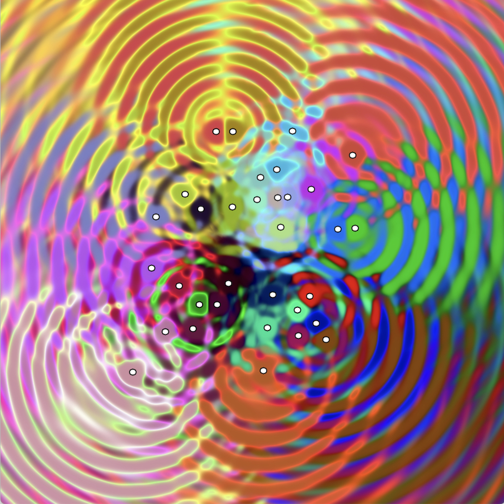
The image below demonstrates how Tölvera's state and drawing capabilities can be used to enable real-time visualisation of IML mappings.
Computer Vision (tv.cv)
Tölvera integrates with OpenCV and Mediapipe to enable exploration of computer vision and tracking of hands, face and full body pose. See examples.
Command-line arguments
When Tölvera is instanced, a global kwargs dictionary is passed down through the various modules that allows setting of flags and parameters.
Tölvera Module (python -m tolvera)
All arguments below can be applied, and in addition:
See also sketchbook in experiments.
Tölvera Context (tv.ctx)
Tölvera Instance (tv)
--name          Name of Tölvera instance. Defaults to "Tölvera".
--speed         Global speed scalar. Defaults to 1.
--particles     Number of particles. Defaults to 1024. Aliased to tv.pn.
--species       Number of species. Defaults to 4. Aliased to tv.sn.
--substep       Number of substeps of render function. Defaults to 1.
Taichi (tv.ti)
--gpu        GPU architecture to run on. Defaults to "vulkan".
--cpu        Run on CPU instead of GPU. Defaults to False.
--fps        Frames per second. Defaults to 120.
--seed       Random seed. Defaults to int(time.time()).
--headless   False
--name       Instance name. Defaults to "Tölvera".
Pixels (tv.px)
--polygon_mode  Polygon drawing mode. Defaults to 'crossing'.
--brightness    Brightness scalar. Defaults to 1.
Open Sound Control (tv.osc)
--osc               Enable OSC. Defaults to False.
--host              OSC Host IP. Defaults to "127.0.0.1".
--client            OSC Client IP. Defaults to "127.0.0.1".
--client_name       OSC client name. Defaults to self.ctx.name_clean.
--receive_port      OSC host port. Defaults to 5001.
--send_port         OSC client port. Defaults to 5000.
--osc_trace         Print all OSC messages. Defaults to False.
--osc_verbose       Verbose printing of iipyper. Defaults to False.
--create_patch      Create a Max or Pd patch based on tv.osc.map. Defaults to False.
--patch_type        Type of patch to create. Defaults to "Pd".
--patch_filepath    Filepath of patch. Defaults to self.client_name.
--export_patch      Export patch schema to XML, JSON or both. Defaults to None.
Interactive Machine Learning (tv.iml)
--update_rate           Rate of IML updates relative to FPS. Default to 10.
--config                anguilla instance configuration. Default to {}.
--map_kw                anguilla.map kwargs. Default to {}.
--infun_kw              Input method kwargs. Default to {}.
--outfun_kw             Output method kwargs. Default to {}.
--randomise             IML randomisation. Default to False.
--rand_pairs            IML randomisation. Default to 32.
--rand_input_weight     IML input randomisation weight. Default to None.
--rand_output_weight    IML output randomisation weight. Default to None.
--rand_method           IML randomisation method. Default to "rand".
--rand_kw               IML randomisation kwargs. Default to {}.
--lag                   Lag value updates. Default to False.
--lag_coef              Lag coefficient. Default to 0.5.
--name                  Name of IML instance. Default to None.
Computer Vision (tv.cv)
--camera            Enable camera. Defaults to False.
--device            OpenCV device index. Defaults to 0.
--substeps          Number of substeps for reading camera frames. Defaults to 2.
--colormode         Color channels. Defaults to 'rgba'.
--ggui_fps_limit    FPS limit of Taichi GGUI. Defaults to 120fps.
--hands             Enable hand tracking. Defaults to False.
--pose              Enable pose tracking. Defaults to False.
--face              Enable face tracking. Defaults to False.
--face_mesh         Enable face mesh tracking. Defaults to False.